Shrinkage in DESeq2
DESeq2 is a popular bioinformatics tool for identifying differentially expressed genes from RNA-Seq data.
In DESeq2, the calculation of log2 fold changes (LFC) is a key step. However, LFC can be misleading, particularly with extreme fold changes for genes with low counts or high variability.
DESeq2 addresses this noisy LFC by applying shrinkage to log2 fold changes (implemented as lfcShrink function) to reduce the impact of outliers and making the results more reliable
for ranking and visualization.
The following example explains how to use shrinkage of log2 fold changes using DESeq2.
Load count dataset
We will use the sequence read count data from the pasilla library for performing differential gene expression analysis and applying shrinkage of log2 fold changes.
Load the read count data and sample information table,
# import librar
library("pasilla")

# load count data
counts <- system.file("extdata",
                      "pasilla_gene_counts.tsv",
                      package="pasilla", mustWork=TRUE)

# convert to matrix
counts_mat <- as.matrix(read.csv(counts, sep="\t", row.names="gene_id"))

head(counts_mat)

# output
            untreated1 untreated2 untreated3 untreated4 treated1 treated2 treated3
FBgn0000003          0          0          0          0        0        0        1
FBgn0000008         92        161         76         70      140       88       70
FBgn0000014          5          1          0          0        4        0        0
FBgn0000015          0          2          1          2        1        0        0
FBgn0000017       4664       8714       3564       3150     6205     3072     3334
FBgn0000018        583        761        245        310      722      299      308


# load sample information table
anot <- system.file("extdata",
                       "pasilla_sample_annotation.csv",
                       package="pasilla", mustWork=TRUE)
coldata <- read.csv(anot, row.names=1)
coldata <- coldata[,c("condition", "type")]
coldata$condition <- factor(coldata$condition)

# output
             condition        type
treated1fb     treated single-read
treated2fb     treated  paired-end
treated3fb     treated  paired-end
untreated1fb untreated single-read
untreated2fb untreated single-read
untreated3fb untreated  paired-end
In the read count dataset, we have count data from two conditions viz. treated and untreated samples. The treated and untreated samples have three and four replicates, respectively.
For DESeq2, the column names of the count table and row names of the sample information table must match and be in the same order.
# make column names from count data and row names from sample table similar
rownames(coldata) <- sub("fb", "", rownames(coldata))
all(rownames(coldata) %in% colnames(counts_mat))

# output
[1] TRUE

# make column names from count data and row names from sample table in same order
counts_mat <- counts_mat[, rownames(coldata)]
all(rownames(coldata) == colnames(counts_mat))

# output
[1] TRUE
Construct a DESeqDataSet and set reference level
Construct a DESeqDataSet for differential gene expression analysis using DESeqDataSetFromMatrix function.
In this step, you can also assign the control sample using relevel for calculating the expression changes between treated and untreated samples.
# import library
library("DESeq2")

# construct DESeqDataSet
dds <- DESeqDataSetFromMatrix(countData = counts_mat,
                              colData = coldata,
                              design = ~ condition)

# set untreated as control sample
dds$condition <- relevel(dds$condition, ref = "untreated")
Additionally, you can also apply filtering before differential gene expression analysis to remove the low count genes.
Differential gene expression analysis
Perform differential gene expression analysis using DESeq
dds <- DESeq(dds)
res <- results(dds)
res

head(res)
# output

log2 fold change (MLE): condition untreated vs treated
Wald test p-value: condition untreated vs treated
DataFrame with 6 rows and 6 columns
               baseMean log2FoldChange     lfcSE        stat    pvalue      padj
              <numeric>      <numeric> <numeric>   <numeric> <numeric> <numeric>
FBgn0000003    0.171569    -1.02604541  3.805503 -0.26962147 0.7874515        NA
FBgn0000008   95.144079    -0.00215142  0.223884 -0.00960955 0.9923328  0.996927
FBgn0000014    1.056572     0.49673557  2.160264  0.22994204 0.8181368        NA
FBgn0000015    0.846723     1.88276170  2.106432  0.89381546 0.3714206        NA
FBgn0000017 4352.592899     0.24002523  0.126024  1.90459450 0.0568328  0.282361
FBgn0000018  418.614931     0.10479911  0.148280  0.70676360 0.4797134  0.823907
The output reports log2 fold changes (log2FoldChange), p value (pvalue), and adjusted p value (padj).
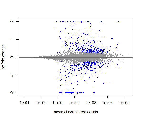
Visualize the differential gene expression using MA plot,
plotMA(res, ylim=c(-2,2))
Shrinkage of log2 fold changes
The low count or highly variable count genes could impact the true estimation of log2 fold changes and can lead to unreliable results.
In this case, you can use shrinkage of log2 fold changes using lfcShrink function for reducing the impact of extreme fold changes and making the results more reliable for ranking and visualization.
The lfcShrink function needs a coefficient that we want to shrink, which can be obtained by resultsNames function.
resultsNames(dds)

# output
[1] "Intercept"                      "condition_untreated_vs_treated"
Perform shrinkage of log2 fold changes for condition_untreated_vs_treated comparison,
resLFC <- lfcShrink(dds, coef="condition_untreated_vs_treated", type="apeglm")

head(resLFC)

# output
log2 fold change (MAP): condition untreated vs treated
Wald test p-value: condition untreated vs treated
DataFrame with 6 rows and 5 columns
               baseMean log2FoldChange     lfcSE    pvalue      padj
              <numeric>      <numeric> <numeric> <numeric> <numeric>
FBgn0000003    0.171569   -0.007217218  0.205803 0.7874515        NA
FBgn0000008   95.144079   -0.000798434  0.151704 0.9923328  0.996927
FBgn0000014    1.056572    0.004660654  0.204893 0.8181368        NA
FBgn0000015    0.846723    0.018121745  0.206169 0.3714206        NA
FBgn0000017 4352.592899    0.190154460  0.120136 0.0568328  0.282361
FBgn0000018  418.614931    0.070624117  0.123741 0.4797134  0.823907
In the above example, we have used the apeglm function for effect size shrinkage. The apeglm is the default estimator in DESeq2.
In addition, you can also use ashr and normal methods for shrinkage estimation.
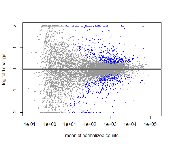
Visualize the differential gene expression after shrinkage of log2 fold changes using MA plot,
plotMA(resLFC, ylim=c(-2,2))

If you compare the MA plot with and without shrinkage of log2 fold changes, you can see that with shrinkage the extreme points are pulled towards the center, making it easier to identify truly differentially expressed genes while reducing the noise from low-count genes.
